Interfacing Fortran and Python for ODE Modeling: A Performance Study on Ethylene Dichloride Cracking

1. Introduction

This project explores the integration of Fortran and Python to solve a system of ordinary differential equations (ODEs) modeling the thermal cracking of Ethylene Dichloride (EDC), a process used in vinyl chloride production. The goal is to benchmark a compiled Fortran solver wrapped via f2py against a pure Python implementation using the same numerical algorithm.

The work builds upon Dr. Helianildes Silva Ferreira’s doctoral research on EDC kinetics and revisits the same reaction system with a modern mixed-language approach.

2. Reaction System and Mathematical Model

The thermal cracking of EDC is represented by two consecutive first-order reactions:

\[ A (\text{EDC}) \xrightarrow{k_1} B (\text{intermediate}) \xrightarrow{k_2} C (\text{product}) \]

The corresponding ODE system is:

\[ \frac{d[A]}{dt} = -k_1[A], \quad \frac{d[B]}{dt} = k_1[A] - k_2[B], \quad \frac{d[C]}{dt} = k_2[B] \]

For this study, we use rate constants \(k_1 = 1.0\) and \(k_2 = 0.5\).

3. Numerical Method: Runge–Kutta–Gill (RKG)

The Runge–Kutta–Gill method is a fourth-order integration technique similar to the classical RK4 but with coefficients that reduce round-off error.

Coefficients used:

\[ A = \frac{\sqrt{2} - 1}{2}, \quad B = \frac{2 - \sqrt{2}}{2}, \quad C = -\frac{\sqrt{2}}{2}, \quad D = \frac{2 + \sqrt{2}}{2} \]

At each step:

\[ y_{i+1} = y_i + \frac{h}{6}(K_1 + K_4) + \frac{h}{3}(B K_2 + D K_3) \]

where the increments \(K_1, K_2, K_3, K_4\) are derived from successive evaluations of the derivative function.

4. Fortran Implementation (fortran-code.f90)

The core numerical solver is implemented in Fortran for performance and compiled into a Python module (cracker) using f2py.

subroutine rk4g_solver(n, h, y0, y_out)
    implicit none
    integer, intent(in) :: n
    real*8, intent(in) :: h
    real*8, intent(in) :: y0(3)
    real*8, intent(out) :: y_out(3, n+1)

    real*8 :: A, B, C, D
    real*8 :: K1(3), K2(3), K3(3), K4(3)
    real*8 :: y(3)
    integer :: i

    A = (sqrt(2.d0) - 1.d0)/2.d0
    B = (2.d0 - sqrt(2.d0))/2.d0
    C = -sqrt(2.d0)/2.d0
    D = (2.d0 + sqrt(2.d0))/2.d0

    y = y0
    y_out(:, 1) = y0

    do i = 1, n
        call f(y, K1)
        call f(y + 0.5d0*h*K1, K2)
        call f(y + h*(A*K1 + B*K2), K3)
        call f(y + h*(C*K2 + D*K3), K4)

        y = y + (h/6.d0)*(K1 + K4) + (h/3.d0)*(B*K2 + D*K3)
        y_out(:, i+1) = y
    end do
end subroutine rk4g_solver

The derivative function f(y, dy) defines the ODE system with constants \(k_1 = 1.0\), \(k_2 = 0.5\).

5. Python Integration (ftp.py)

The Fortran code is exposed to Python via f2py and dynamically loaded. A short simulation with 100 steps and step size h = 0.1 produces the expected concentration profiles.

import importlib.util
import numpy as np
import matplotlib.pyplot as plt

path = "./cracker.cpython-312-darwin.so"
spec = importlib.util.spec_from_file_location("cracker", path)
cracker = importlib.util.module_from_spec(spec)
spec.loader.exec_module(cracker)

h = 0.1
n_steps = 100
y0 = np.array([1.0, 0.0, 0.0], dtype=np.float64)
y_out = cracker.rk4g_solver(n_steps, h, y0)

z = np.linspace(0, h * n_steps, n_steps + 1)
plt.plot(z, y_out[0], label="EDC")
plt.plot(z, y_out[1], label="MVC")
plt.plot(z, y_out[2], label="HCl")
plt.xlabel("z")
plt.ylabel("Concentration")
plt.title("Thermal Cracking of EDC (Fortran + Python)")
plt.legend()
plt.grid(True)
plt.show()

6. Pure Python Version

A Python-only version implements the same RKG algorithm and kinetic system using NumPy arrays. It follows identical logic but executes within Python’s interpreter, leading to slower runtime due to loop overhead.

7. Benchmarking

Benchmarks are run for various step counts:

ns = [100, 500, 1000, 2000, 5000, 10000, 20000, 50000, 100000, 200000, 500000, 1000000]

Each n corresponds to the number of integration steps. With a fixed step size \(h = 0.1\), total simulated time is \(T = n \times h\).

for n in ns:
    tf = timeit.timeit(lambda: run_fortran(n), number=5)
    tp = timeit.timeit(lambda: run_python(n), number=5)
    print(f"n={n} | Fortran: {tf:.4f}s | Python: {tp:.4f}s | Speedup: {tp/tf:.2f}x")

8. Implementation Details

The workflow connecting Fortran and Python consists of four main stages, illustrated below.

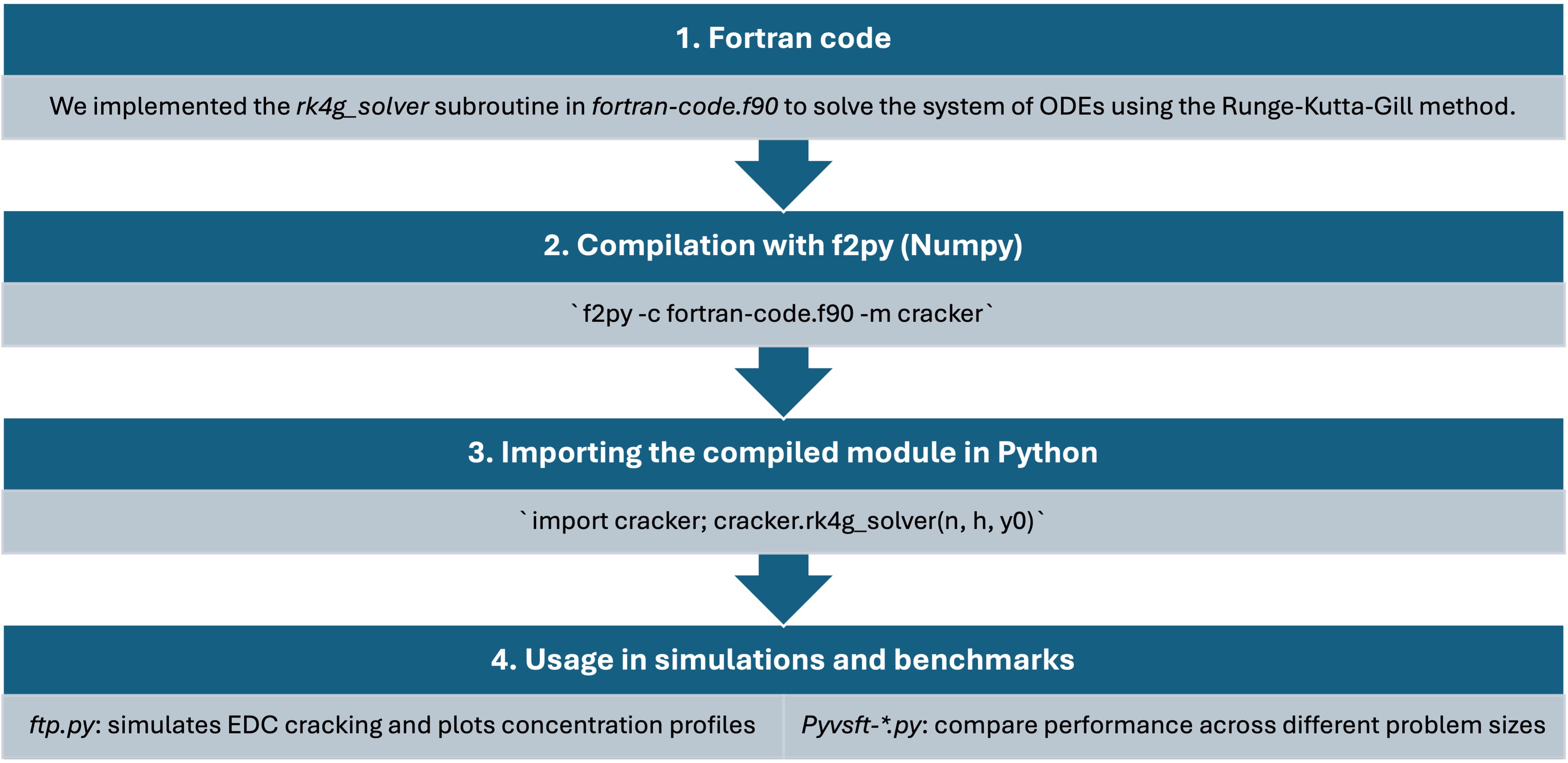
1. Fortran code

We implemented the rk4g_solver subroutine in fortran-code.f90 to solve the system of ODEs using the Runge–Kutta–Gill method. This subroutine computes the concentrations of A, B, and C at each integration step.

2. Compilation with f2py (NumPy)

The Fortran subroutine is compiled into a Python-compatible shared library using f2py:

f2py -c fortran-code.f90 -m cracker

This produces a binary module (cracker.so or .pyd) that can be imported directly into Python.

3. Importing the compiled module in Python

After compilation, the module is loaded and the subroutine is called from Python:

import cracker
cracker.rk4g_solver(n, h, y0)

This call executes the compiled Fortran code from within Python, allowing numerical results to be returned as NumPy arrays.

4. Usage in simulations and benchmarks

• ftp.py — simulates the EDC cracking process and plots concentration profiles.
• pyvsft-basic_example.py — compares execution time between Fortran and Python solvers for a fixed problem size.
• pyvsft-with_steps.py — performs scaling benchmarks across increasing step counts (n values) to measure performance trends.

Together, these scripts illustrate the complete mixed-language workflow: Fortran for computation and Python for analysis, visualization, and benchmarking.

9. Results

Simulation Results

The coupled Fortran–Python implementation accurately reproduces the expected kinetic behavior of the thermal cracking of 1,2-dichloroethane (EDC).

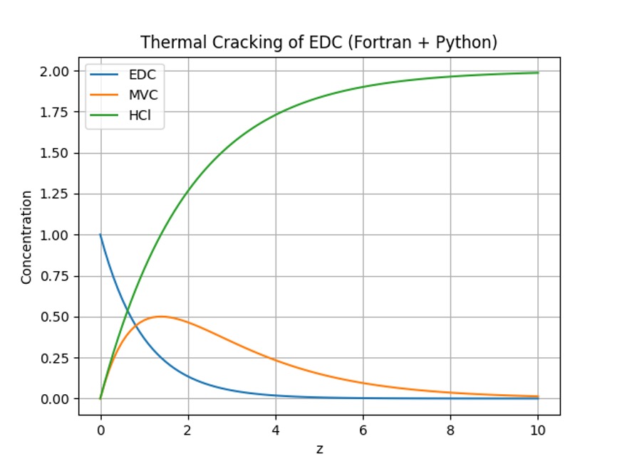
Figure 1. Concentration profiles for EDC (A), MVC (B), and HCl (C) as a function of the reaction coordinate z.

• EDC (A) decreases exponentially, indicating its consumption as the primary reactant.
  
• MVC (B) appears transiently, reaching a maximum concentration before decomposing further.
  
• HCl (C) accumulates continuously as a stable final product.

The agreement between the Fortran and Python implementations validates the correctness of the rk4g_solver algorithm and confirms consistent numerical accuracy.

---

Performance Benchmarks

Runtime measurements demonstrate the efficiency gains achieved by executing the Runge–Kutta–Gill method in compiled Fortran versus interpreted Python.

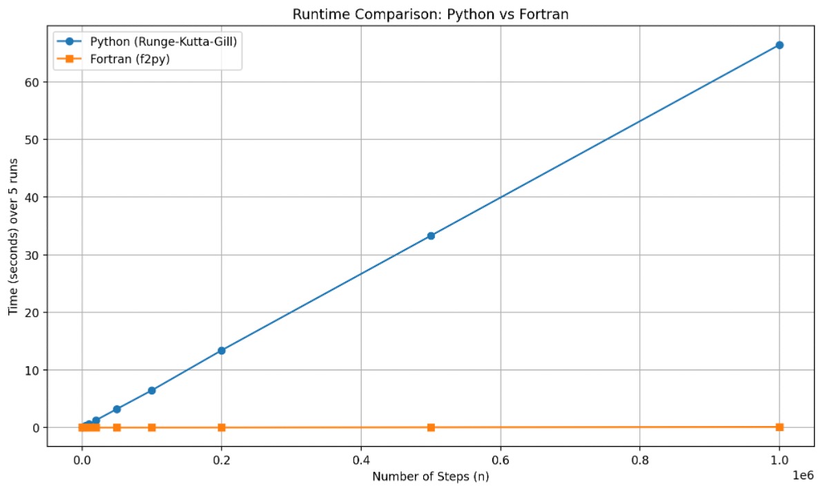
Figure 2. Runtime comparison between Fortran (f2py) and Python (Runge–Kutta–Gill) solvers for increasing numbers of integration steps (n).

• Fortran’s runtime remains nearly constant, even at large n, showing excellent scalability.
  
• Python’s runtime increases linearly due to loop interpretation overhead.
  
• At one million steps, Fortran outperforms Python by approximately 700×.

For more details, see the table below:

n	Fortran Time (ms)	Python Time (ms)	Speedup (x)
100	0	6.0	230.84
500	0	30.0	613.93
1000	0.1	60.0	570.25
2000	0.2	118.7	660.38
5000	0.4	302.1	680.40
10000	1.0	618.5	638.93
20000	1.8	1283.8	722.32
50000	4.5	3228.8	723.16
100000	9.7	6465.2	669.15
200000	19.3	13402.7	695.66
500000	48.8	33289.5	682.82
1000000	94.8	66422.6	700.39

Table 1. Fortran is always faster than Python for this ODE integration task, with speedups exceeding 200x even for small step counts and reaching over 700x for large simulations.

This highlights the advantage of mixed-language workflows, where Fortran handles computation-intensive loops and Python facilitates benchmarking and visualization.

---

Discussion

The results confirm:

• Numerical accuracy: Both solvers produce identical concentration profiles.
  
• Performance scalability: Fortran maintains low runtime even for large problem sizes.
  
• Integration benefit: Using f2py bridges Fortran’s computational efficiency with Python’s usability.

These findings illustrate the practical application of mixed-language workflows between legacy scientific languages and modern scripting tools, emphasizing the value of interoperability in computational research.

10. Interpretation

Language	Strength	Limitation
Fortran	Computational efficiency, deterministic performance	Less flexible for data visualization
Python	Rapid prototyping, data analysis, visualization	Slower loops, interpreter overhead

This experiment shows how combining both enables performance + usability, which is a key value in modern computational research.

11. Conclusion

This study demonstrates how f2py enables seamless integration of high-performance Fortran solvers with Python’s ecosystem for visualization and analysis. The results confirm that hybrid workflows preserve legacy numerical power while embracing modern flexibility.

Bigger question: How can we bridge generations of scientific computing, enabling mixed-language workflows?

References

This project was inspired by prior studies that modeled the cracking of Ethylene Dichloride (EDC), particularly:

• Ferreira, H. S. (2003).
  Métodos matemáticos em modelagem e simulação do craqueamento térmico do 1,2-Dicloroetano.
  Doctoral dissertation, University of Campinas, Brazil.
  https://repositorio.unicamp.br/Busca/Download?codigoArquivo=477111

• Schirmeister, R., Kahsnitz, J., & Träger, M. (2009).
  Influence of EDC cracking severity on the marginal costs of vinyl chloride production.
  Industrial & Engineering Chemistry Research, 48(6), 2801–2809.
  https://doi.org/10.1021/ie8006903

• Fahiminezhad, A., Peyghambarzadeh, S. M., & Rezaeimanesh, M. (2020).
  Numerical Modelling and Industrial Verification of Ethylene Dichloride Cracking Furnace.
  Journal of Chemical and Petroleum Engineering, 54(2), 165–185.
  https://doi.org/10.22059/jchpe.2020.286558.1291